Going with the Flow

Notes on Flow Matching (Policies)

December 9, 2024

Note: Flow matching has been added to my diffusion codebase.

Flow Matching

Flow matching is a technique to train neural networks that can iteratively refine an input towards some target, much like diffusion models. I recently came across them in a very interesting paper called One Step Diffusion via Shortcut Models, and implemented flow matching policies on my way to implementing the ideas described in the paper. The first time I encountered flow matching I found the available explanations somewhat convoluted, so I wanted to (1) try explaining my understanding of flow matching on its own, (2) take a look at flow matching policies, and finally (3) look at some results from applying them. In a follow-up post I will discuss shortcut models.

My best intuition for flow matching is that instead of training a network to model some function $f (x)$ , we instead want to model its derivative $f^{'} (x)$ . When we feed some input $x$ into our network, it therefore does not tell us the intended answer $y$ , but instead tells us how $x$ could be changed to approach $y$ . If we iterated through this network many times, we could manually walk our data point $x$ towards $y$ until we think we have reached it. You could also call this process "integration" or "Euler's Method".

Using a Flow Matching Model

Given an initial datapoint $x_{0}$ and a flow matching model $f^{'} (x)$ :
Repeat:
1. use the model to output $v = f^{'} (x)$ locally at $x_{i}$
2. update our datapoint: $x_{i + 1} = x_{i} + (v * s t e p_{s} i z e)$

As far as I can tell, this really only makes sense if $x$ and $y$ are the same shape and we can imagine mapping from one to the other. Usually $x_{0}$ is a sample from a random normal with the same shape as $y$ .

The main question is how to determine our training data and our step size above. While there are lots of options, the most straightforward is to have the model output the difference between $y$ and the corresponding $x_{0}$ . This has the nice property that the output of the model is proportional to magnitudes within the data, and thus our step size can be considered a fraction of this difference. For example, if our step_size is some small quantity like 0.01, that would mean "move 1% of the original distance to y". In this case, we would therefore iterate for 100 steps.

To train this model, we need to make two changes from a typical neural network regression task: Firstly, our training target is not $y$ itself, but $(y - x)$ : given some $x$ , can we predict the vector pointing from $x$ to $y$ ? Secondly, since we will be using the model at many intermediate points between some $x_{0}$ and $y$ , we need it to be familiar with all these points as well. So, more accurately: Given some $(x_{t}, t)$ where $t$ is between 0 and 1, can we predict $(y - x_{0})$ ? In our training loop, we can construct these intermediate points by interpolation, giving us:

Flow Matching Training

Given some $(x_{0}, y)$ pair:
Sample some $t$ between 0 and 1, possibly from a discrete set of options.
Construct $x_{t} = y * t + x_{0} * (1 - t)$
Update the network such that $N e t w o r k (x_{t}, t)$ predicts $(y - x_{0})$

Flow Matching as Vector Fields

Many explanations of flow matching describe it as "modeling a vector field": for a fixed time $t$ , we could pass in any input and would receive as output a corresponding vector telling us in what direction to adjust our input, with a magnitude given by our step size. If we visualized the outputs for the space of possible inputs (and a fixed time $t$ ), we would see a vector field.

Note that this is conditional on $t$ , so the vector field changes at each time step. During inference, by updating our inputs according to the corresponding vector, we are "flowing" a point through this changing vector field. If successful, our network has learned to "match the flow" of this process which maps points in $P (X)$ to points in $P (Y)$ .

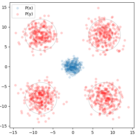
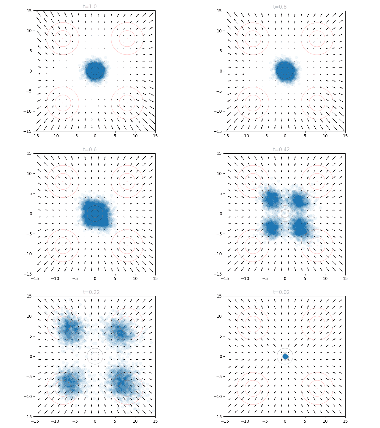
This is best visualized with a problem in 2D space. Suppose we want to generate points from a distribution given by four gaussians, one in each quadrant, at (8,8), (-8,8), (8,-8), and (-8,-8). This will be our target distribution $P (Y)$ . We will instead sample from the standard normal around (0,0), our starting distribution $P (X)$ . Concentric circles show mean (center dot), one standard deviation, and two standard deviations:

We can train a neural network to output a vector field that moves the points in $P (X)$ to $P (Y)$ over many timesteps, as described above. The input to our network is therefore a 2D point and a timestep $t$ , and the output is a vector. We can visualize the vector field at a given $t$ by sweeping over a grid of points and plotting the resulting vectors. If we repeat this for many $t$ from 0 to 1, we can see how the vector field changes over time.

plot_animation_vf

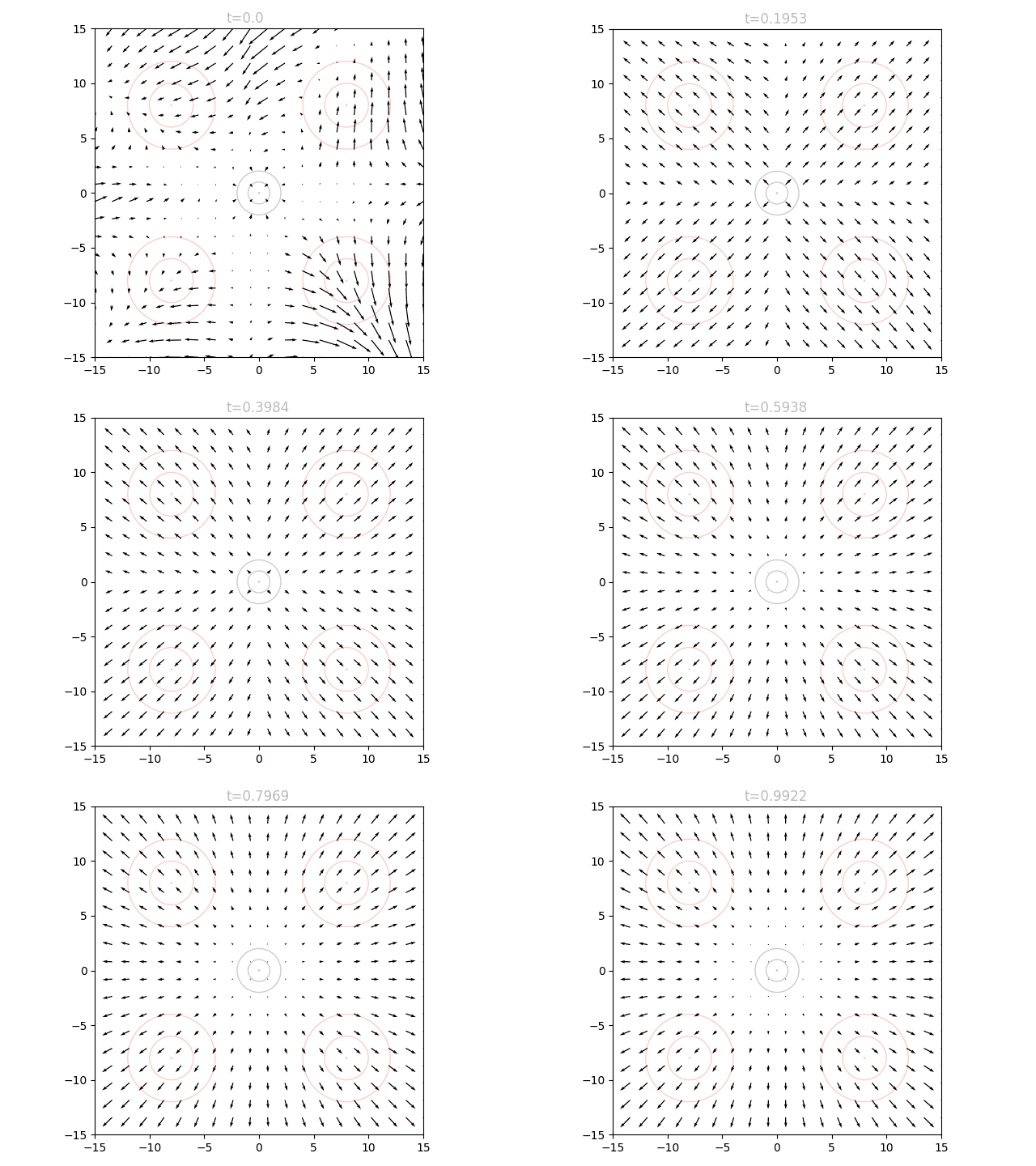
We can see that initially the vector field far the origin is fairly wonky, since no relevant points will be out there yet and it is quite literally "out of distribution". We can also see that as $t$ approaches 1.0, the vectors around the origin become very small in magnitude. This is for a similar reason: as our points approach the final distribution, we should no longer have points near the center.

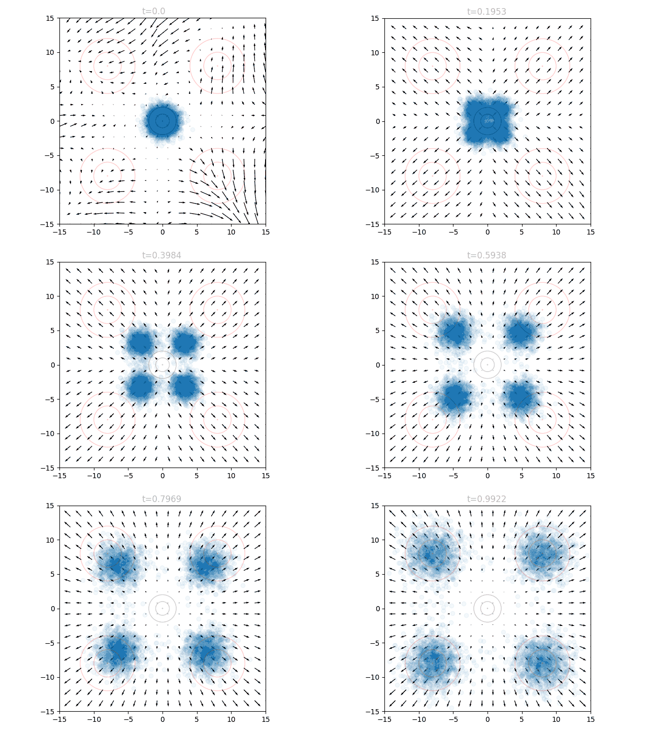
To actually use our network, we initialize points from $P (X)$ and set $t = 0$ . We can query the network for the local vectors at each point, and use this to update the points. We then increase $t$ slightly, and repeat. This can be visualized as an animation, here showing 5k points as well as the underlying vector field:

plot_animation

Breaking Changes

To help understand why we are going to all this trouble to model $f^{'} (x)$ , and condition our model on $t$ , we can look at what happens if we don't do this.

Firstly, if we try to create a network that takes in a point in $x$ and outputs a point in $y$ (directly regressing on random (x,y) pairs), we don't get very far. Since there is no clear mapping between the two distributions, our network just learns the average:

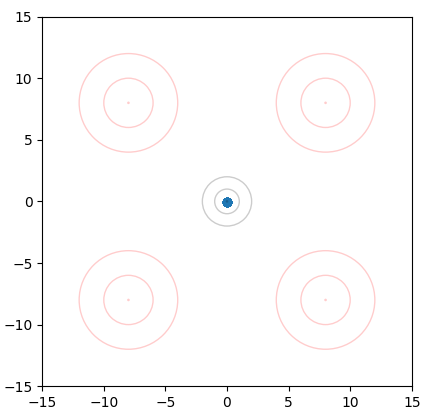
The blue dot is actually 5k points stacked on top of each other.

Another question to consider is why the inclusion of $t$ ? If we look at our animation in the previous section, the vector field doesn't change very much, and we could certainly imagine a static vector field that flows the points properly. This is actually what you get if you don't train for very long, and the model doesn't yet fit to which areas of the space are occupied. I think this is also the reason why we include t: it allows the model to focus on relevant areas of the data space during our generation, and ignore areas where most points will not reside. This is not very critical for our example problem, but I can imagine this being important for very complex generation tasks.

Flow Matching vs Diffusion

The process of flow matching is incredibly similar to diffusion, and depending on your specific setup they may be indistinguishable. A diffusion model in image generation is often described as predicting the noise that might be present in an image, so that the noise can be subtracted away. From the DDPM paper we see the following:

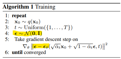
We generate random noise at step 4, and then try to predict the noise at step 5. In step 5, we are minimizing the squared error between the actual noise (epsilon) and our model's output (epsilon sub theta).

Another way to formulate this would be to take a clean image, add noise to get a noisy image, and then subtract the two. You would be left with the noise itself! Therefore, predicting noise in diffusion is the same idea as predicting the difference between samples in flow matching. The difference is really just in how to formulate the problem: in diffusion we predict noise and subtract it away, in flow matching we predict a change and add it on.

The more substantial difference between flow matching and diffusion is in the trajectories that datapoints take when moving from P(X) to P(Y). Diffusion models use a schedule that does not necessarily move $x$ straight towards $y$ or at a uniform rate. DDPM uses a schedule that updates data in a sigmoid(ish) fashion, initially taking small steps, then large ones, then slowly converging to the desired point:

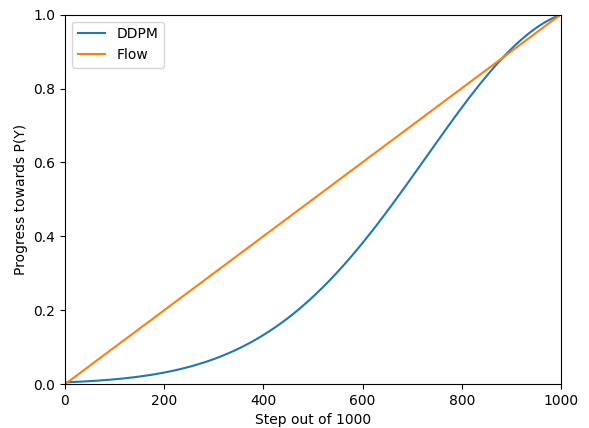
The blue line is generated by running the DDPM diffusion process on a value at 1.0 towards a value of 0.0, and then flipping this around to approximate "generation".

The shape of this line is reflected when we visualize the "vector field" of a diffusion model on our same problem. Rather than flowing linearly, the points accelerate towards the final distribution:

plot_animation_diffusion

Uniting Flow Matching and Diffusion Codebases

Fortunately, since the objectives and input/output are quite similar, we can reuse a diffusion implementation to achieve flow matching with minimal changes. In my diffusion policies repository, I recently abstracted away the algorithm to try uniting these frameworks. It is helpful to revisit each in pseudocode:

DDPM : Clean Sample to Noisy Point

Given datapoint y, timestep t, and random noise sample $ϵ$ :

Retrieve $\bar{a}$ from the diffusion schedule
$x_{t} = \sqrt{\bar{a}} * y + \sqrt{1 - \bar{a}} * ϵ$
Update the model to minimize the MSE between $ϵ$ and $M o d e l (x_{t})$

Flow Matching: Clean Sample to Noisy Point

Given datapoint y, timestep t, and random noise sample $ϵ$ :

$x_{t} = t * y + (1 - t) * ϵ$
Compute target: $y - ϵ$
Update the model to minimize the MSE between target and $M o d e l (x_{t})$

We have something similar in generation: Our model will predict some noise, and we can defer to each algorithm how that prediction will be used to update the datapoint. One critical gotcha is that during generation, diffusion considers the "diffusion process" to be going in reverse, starting at T=100% (noise) and approaching T=0% (clean), whereas flow matching may treat T in the opposite fashion, starting at 0. It is also a headache to keep track of T in whole steps (diffusion) versus fractional steps out of 1.0 (flow matching). All of these boil down to personal implementation preferences but just be aware that it is an easy area to introduce a bug.

In code we can keep all of this separated in algorithm classes that manage these details; I will show a snippet here of the recently refactored codebase:


class DDPMAlgo():



    def __init__(self, T, **kwargs):

        self.T = T

        self.betas = np.linspace(0.0001, 0.02, T)

        self.alphas = 1.0 - self.betas

        self.alpha_hats = np.cumprod(self.alphas)

        self.ts = list(range(self.T))

        self.sampling_d = None

        self.reverse_gen = True # we run our T's in reverse order to generate



    def forward_diffusion(self, data, noise, t):

        '''

        Given the unnoised data, a noise tensor of same size, and an integer index t

        returns: (the noised data point, the MSE training target)

        '''

        ahat = self.alpha_hats[t.detach().cpu().numpy()]

        ahat = torch.as_tensor(ahat).to(torch.float32).to(data.device)

        B, d1, d2 = data.shape

        ahat = ahat.unsqueeze(1).unsqueeze(2).repeat(1,d1,d2)

        noised_batch = torch.sqrt(ahat)*data + torch.sqrt(1.0 - ahat)*noise

        return noised_batch, noise



    def generation(self, x, t, pred_noise):

        '''

        Given a partially refined datapoint x, the time t, and a prediction from our model,

        update and return the new x.

        '''

        z = torch.randn(*x.shape).to(torch.float32).to(self.device)

        if t == 0:

            z *= 0

        beta = self.betas[t]

        alpha = self.alphas[t]

        alphahat = self.alpha_hats[t]

        x = (1.0/math.sqrt(alpha))*(x - ((1.0 - alpha)/math.sqrt(1.0 - alphahat))*pred_noise) + math.sqrt(beta)*z

        return x





class FlowMatchingAlgo():

    def __init__(self, T, step_size=20, **kwargs):

        self.T = T

        self.step_size = step_size

        self.ts = list(range(self.T))[::step_size]

        self.sampling_d = int(np.log2(step_size))

        self.reverse_gen = False



    def forward_diffusion(self, data, noise, t):

        t_fractional = t.to(torch.float32) / float(self.T)

        _, d1, d2 = data.shape

        t_fractional = t_fractional[:,None,None].repeat(1,d1,d2)

        noised_batch = (1.0-t_fractional)*noise + t_fractional*data

        velocity = data - noise

        return noised_batch, velocity



    def generation(self, x, t, pred_noise):

        # here the "predicted noise" is more accurately "velocity"

        # we need to multiply by a scalar to get the appropriate change to x.

        velocity = pred_noise

        step_size_fractional = float(self.step_size)/float(self.T)

        x = x + velocity*step_size_fractional

        return x

Flow Matching Policies on CarRacing-v3

We swap out flow matching as our algorithm of choice when creating a diffusion policy (I guess now a flow matching policy). Just like diffusion policies, we can use a UNet architecture and we make our network conditional on an observation: rather than Model(x, t) predicting a change in x, we now have Model(x, t, c) predicting that change.

$x$ is some tensor with the same size as a sequence of actions from an environment. Starting with random noise, we "flow" this tensor towards a generated snippet of actions which make sense given the current observation ( $c$ above). Just like diffusion policies, our training data comes from a series of expert trajectories. Our goal is thus to generate actions, conditioned on observations, that would be drawn from the output distribution of the expert "policy", approximated here by data.

My markdown converter is misbehaving so what I intended to be a table will have to be a list.

DDIM, 50 Step Generation:
- Performance: 883.6 +/- 151.4 on average, 919.8 +/- 3.0 for middle 50% of episodes.
- FPS: 12.0, drops to 3.0 on generation steps
DDIM, 10 Step Generation:
- Performance: 910.0 +/- 50.8 on average, 921.9 +/- 3.1 for middle 50% of episodes.
- FPS: 51.0, drops to 12.8 on generation steps
Flow Matching, 50 Step Generation:
- Performance: 897.3 +/- 84.8 on average, 920.9 +/- 4.8 for middle 50% of episodes.
- FPS: 12.5, drops to 3.1 on generation steps
Flow Matching, 10 Step Generation:
- Performance: 890.6 +/- 119.3 on average, 921.2 +/- 4.6 for middle 50% of episodes.
- FPS: 53.4, drops to 13.4 on generation steps
Expert Performance: 923.8 +/- 8.5

In general, the flow matching policy performed very well, and it is much easier to implement (in my opinion) than diffusion. All versions of both policies generally matched the expert ability.

In practice, a key limitation of these methods is needing to pause periodically to generate new actions, and this is reflected in the last column. If we assume this generation is the bottleneck for FPS, and we use this FPS for all actions to enforce smooth movement, what is the effective actions per second? If we do not care about smoothness, we can average out the FPS, seen in the second-to-last column.

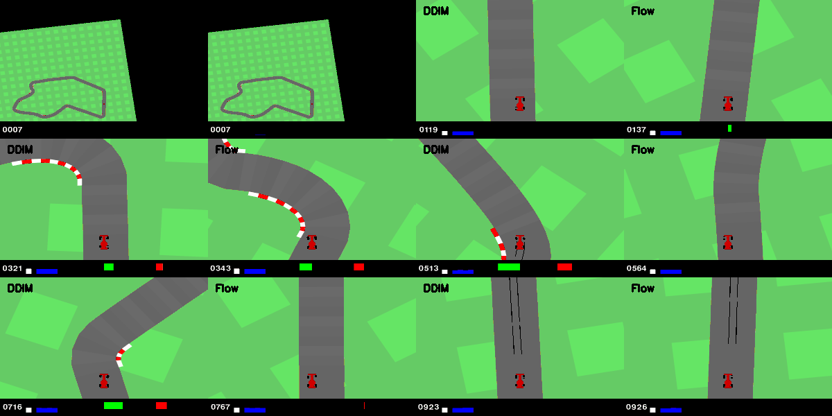
Finally, some results animations:

small_animation

I am going to follow this post with a parallel write-up on shortcut models, which I have found to perform similarly to these techniques but overcome many annoyances in deployment.

Update: that post is here.