Flowing with Fewer Steps

Shortcut Models Notes and Review

December 12, 2024

Note: Shortcut models have been added to my diffusion codebase.

Shortcut Policies

In previous posts I have looked at flow matching and diffusion as a basis for imitating expert policies, and they perform really well (much better than behavior cloning). However, they do have a key limitation: inference speed. To deploy a policy that is based on either of these methods, we may need to perform 10s or 100s of inference passes to generate the next few actions, and this makes it hard to use a policy that requires a quick reaction time. For example, an autonomous vehicle would not perform very well if needed to "stop and think" every few seconds while going 65 mph on the highway. In fact, in my previous examples using CarRacing-v3, I had to post-process the results videos for this exact reason- the live version is very choppy and hard to watch.

This is also a problem in image generation, where many of the ideas in these methods originated. If I want to deploy a service that lets users generate an image, but every query requires 50 passes through my giant model, my service is either going to painfully slow or my AWS bill is going to be very high.

Fortunately, there are a variety of methods to mitigate this problem between training and deployment- we can distill the results of our flow matching model (interchangeable with diffusion for the rest of this post) into a new model that mimics this in one (or very few) steps. This is at first glance a little strange: the whole point of flow matching is to help the model learn how to generate over many steps, because a single step is probably not possible. We cannot learn a model that directly regresses on a point of random noise mapped to a point in our desired distribution. If we try this, the model will just learn some sort of average or degraded output.

However, the reason this doesn't work is not because it is impossible, but because we just do not have a sensible mapping to exploit. Once we have a sensible mapping (provided by a trained flow matching model that can generate samples), we can distill this mapping into a new network that performs it in one pass. So a simple version of this is something like:

Given a trained flow matching model:

Sample random noise x.
Over many inference passes, generate a corresponding datapoint y and compute the final delta from x.
Save (x,dx) as a training pair
Repeat until large dataset acquired, or do this in parallel with the next section.

Then in a new model:

Sample (x,dx) datapoints
Train the new model to predict dx from x.
Generate in one step with y = x + dx

This is process works, but there are two annoying things going on here from a practical perspective: (1) we have to train a second model, and (2), in order to harvest data to train this model we need to do many inference passes. Both of these are alleviated by a recent work called One Step Diffusion via Shortcut Models, which I decided to implement and add to my current diffusion policies / flow matching policies implementation because of the clear practical advantages.

Using a Single Model

Let's start with the first problem: multiple models. To fix this, we can imagine creating a multitask network that holds solutions to both the multistep generation (original flow model) and the one-step generation (distilled flow model). To do this we can introduce a new input that just acts like a switch, telling the network what it should model: should it produce a vector field that will be used over several steps, or a vector field for one step? This gives us something like (not our final version):

Model(x, t, d) estimating needed delta x, given:

x, a current noisy datapoint
t, the current timestep in our generation process
d, a switch that indicates if we plan to take many small steps or one large one

We could then train this model using a sort of "self-distillation": as we train the typical flow matching objective when d=0, we also train on the distillation objective and pass d=1:

Self-Distilled Flow Model Training:

Given some $(x_{0}, y)$ pair, compute loss on flow matching objective:
1. Sample some $t$ between 0 and 1, possibly from a discrete set of options.
2. Construct $x_{t} = y * t + x_{0} * (1 - t)$
3. Construct loss1 such that $N e t w o r k (x_{t}, t, d = 0)$ is encouraged to predict $(y - x_{0})$
Given another $(x_{0}, y)$ pair, compute loss on the distillation objective:
1. Outside the computation graph, use the model to generate an expected $y_{g e n}$ over many inference passes
2. Construct loss2 such that $N e t w o r k (x_{0}, t = 0, d = 1)$ is encouraged to predict $(y_{g e n} - x_{0})$
Update on the combined loss: loss1 + loss2

Using Fewer Inference Steps

The second problem of long inference remains, as we can see in 2.1 above. Shortcut Models fixes this by expanding on the above idea. Rather than a binary switch, what if we could construct multiple options that interpolate between our two tasks: many-step generation on one end, one-step generation on the other, and several-step options in the middle. Specifically, shortcut models as described in the paper use 8 options that can be passed in for $d$ : [0,1,2,3,4,5,6,7], indicating that the step size during generation will be $2^{d}$ steps out of a total of 128: [1, 2, 4, 8, 16, 32, 64, 128]. $d = 0$ indicates our typical flow matching case with small steps, while $d = 7$ indicates a single large step.

This is helpful because rather than distilling all the way from many-step distillation to single-step, we can set up a cascading distillation system in which each designated $d$ distills to one step-size higher, and this means we only ever need to take two steps to create a target for distillation. For example, the $d = 1$ case will try to distill two steps of size 1 into a single step of size 2. When d=2, we will try to distill two steps of size 2 into a single step of size 4, and so on:

Shortcut Flow Model Training:

Given some $(x_{0}, y)$ pair, compute loss on flow matching objective:
1. Sample some $t$ between 0 and 1, from increments of 1/128.
2. Construct $x_{t} = y * t + x_{0} * (1 - t)$
3. Construct loss1 such that $N e t w o r k (x_{t}, t, d = 0)$ is encouraged to predict $(y - x_{0})$
Given another $(x_{0}, y)$ pair, compute loss on the distillation objective:
1. Sample some $t$ between 0 and 1, from increments of 1/128.
2. Construct $x_{t} = y * t + x_{0} * (1 - t)$
3. Select some $d_{1}$ at random from [0,1,2,3,4,5,6]
4. Set $d_{2}$ = $d_{1} + 1$
5. Outside the computation graph, take two generation steps forward with $d_{1}$ :
  1. Let $s$ be the corresponding step size for $d_{1}$ in our schedule (i.e. 1, 2, 4, 8, ...)
  2. $x_{t + d}$ = $x_{t}$ + $M o d e l (x_{t}, t, d_{1}) * s$
  3. $x_{t + 2 d}$ = $x_{t + d}$ + $M o d e l (x_{t + d}, t + s, d_{1}) * s$
  4. Compute target velocity = $(x_{t + 2 d} - x_{t}) / 2$
  5. Note that in steps 2 and 3, it is best to use the EMA model if available.
6. Construct loss2 such that $N e t w o r k (x_{t}, t, d = d_{2})$ is encouraged to predict the target velocity
Update on the combined loss: loss1 + loss2

Above, 2.5 is called the "self-consistency loss": generating with two small steps should be equivalent to one step that is twice as large. This self-consistency is performing distillation: Our setting for $d_{i}$ is being distilled from two steps at $d_{i - 1}$ . The paper recommends a data imbalance: perform (1) with a batch size that is 3-5 times larger than the batch size in (2).

The paper also recommends distilling from an EMA model rather than the original: create a second network that tracks an exponential moving average of the weights of the first, and use this for the distillation objective. This is common practice in diffusion and flow matching, so even though it seems like they are introducing a second model, it is sort of assumed that it will exist.

Revisiting our 2D Example

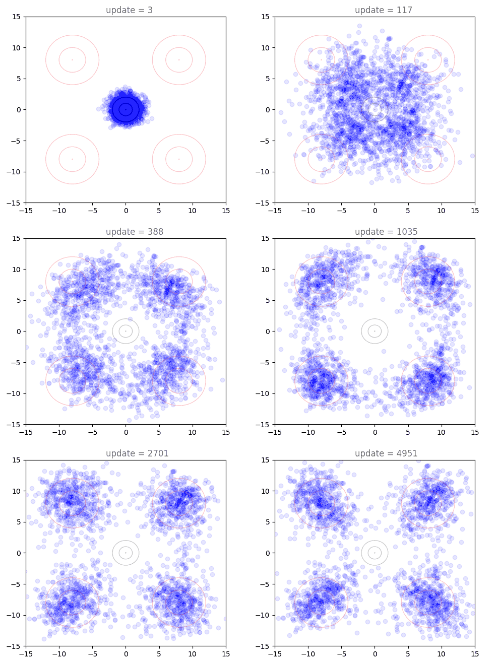
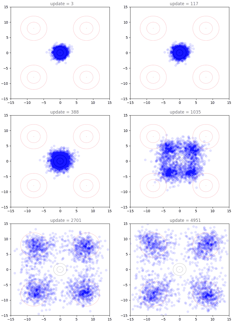
Plotting the training dynamics of shortcut models is really interesting, and it is a non-trivial endeavor to figure out how to visualize this. Even for 2D points, we have 8 separate vector fields that are modelled by the network (depending on choice of $d$ ). To take a look at this, I first want to introduce a new way of looking at our flow matching example from the previous post. The goal is to construct a flow matching model that takes points from a standard normal and flows them to a distribution defined by four wider Gaussians arranged in a cross pattern. Below, we see the results of generating points with our model, over the course of the first 5000 training steps:

one_distribution

This looks very similar to animations of using the flow model itself, but we are looking at something completely different: this shows that as the model trains, it is able to generate points closer and closer to the target distribution. Soon, the target distribution is reached and we see some jitters as the model tries to further refine the boundaries of the distribution. These "jitters" are one reason that diffusion models and flow matching almost always use EMA, a moving average of model weights during training. We can visualize generations under these instead, and they are very smooth:

one_distribution_ema

Our 2D Example with Shortcut Models

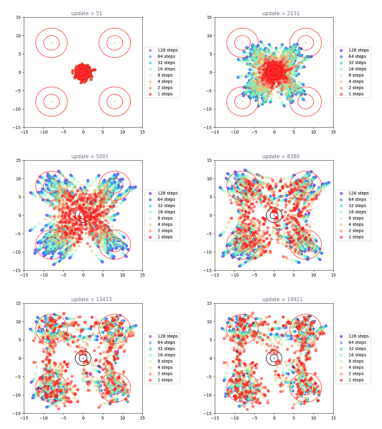
Now we will visualize the same thing, but using a shortcut model. Instead of a single distribution of points, we have 8: one for each of our step sizes defined by $d$ . The standard flow matching objective is used for $d = 0$ , show here in purple (128 steps to generate). Generation under the one-step ( $d = 7$ ) setting is shown in red, with others forming a spectrum in-between:

all_20_smooth

We can directly see the result of the cascading distillation in rainbow streaks that form: the purple points are fastest to train, and the other colors (step sizes) attempt to follow them, each distilling slightly slower than the last. This leads to chains of points through our various settings for $d$ , reaching out towards the intended distribution, and eventually becoming a bit muddier as the model settles. I am very proud of this gif. A version with many more points is used as the cover image, above.

Presumably, as training time tends to infinity, all the points end up on top of each other. However, I never found this to happen in practice, with some "rainbow chains" even in models that trained for a long time.

Shortcut Results on CarRacing-v3

As with diffusion and flow matching, my next step is to use this as the basis of a policy. This is ultimately the advantage of doing some sort of distillation: we can do inference fast. For robotics applications, this may unlock dexterity or maneuvers that would not otherwise be possible at a slow speed.

The shortcut model performed very well on this task, even when using a single step. We see the following performance over 100 episodes:

Shortcut, 128 Step Generation:
- Performance: 861.3 +/- 156.1 on average, 915.5 +/- 9.6 for middle 50% of episodes.
- FPS: 3.5, drops to 0.9 on generation steps
Shortcut, 16 Step Generation:
- Performance: 890.2 +/- 112.2 on average, 916.9 +/- 7.1 for middle 50% of episodes.
- FPS: 27.2, drops to 6.8 on generation steps
Shortcut, 4 Step Generation:
- Performance: 886.1 +/- 105.2 on average, 918.4 +/- 6.0 for middle 50% of episodes.
- FPS: 86.2, drops to 21.6 on generation steps
Shortcut, 1 Step Generation:
- Performance: 893.7 +/- 108.8 on average, 917.3 +/- 4.0 for middle 50% of episodes.
- FPS: 237.5, drops to 59.5 on generation steps
References:
- Expert: 923.8 +/- 8.5
- DDIM 10 Step: 910.0 +/- 50.8, Middle 50%: 921.9 +/- 3.1, FPS 51.0 dropping to 12.8
- Flow 10 Step: 890.6 +/- 119.3, Middle 50%: 921.2 +/- 4.6, FPS 53.4 dropping to 13.4

While the performance is great (pretty much on par with other methods at all step sizes), the key takeaway is in bold underline: At the bottleneck the shortcut policy can run at 60 FPS, and if we average this out we get ~240 FPS. This is also generating 4 actions at a time, which is very conservative. If we generated more I think this could easily surpass 100 FPS, which could enable very precise movements in real time.

As always, some result animations. Here we see DDIM, Flow-Matching, and Shortcut all completing the same track side-by-side:

three_animation

The shortcut model seems like it might be a little choppy in its movement but I am certainly nit-picking. While the first two are post-processed to obtain faster and smoother video, the shortcut model is actually post-processed because it is too fast!

In the future I'd like to apply shortcut models to a more complex problem to see if it remains competitive. I am vert impressed by this method and it will definitely be a technique I use in the future.